Telco Churn

Package Imports

import pandas as pd
import xplainable as xp
from xplainable.core.models import XClassifier
from xplainable.core.optimisation.bayesian import XParamOptimiser
from xplainable.preprocessing.pipeline import XPipeline
from xplainable.preprocessing import transformers as xtf
from sklearn.model_selection import train_test_split
import requests

Instantiate Xplainable Cloud

Initialise the xplainable cloud using an API key from: https://beta.xplainable.io/

This allows you to save and collaborate on models, create deployments, create shareable reports.

xp.initialise(
    api_key="", #<- Add your own token here
)

Out:

VBox(children=(VBox(children=(HBox(children=(HBox(children=(Output(), HTML(value='
        <span style="font-…

Read IBM Telco Churn Dataset

df = pd.read_excel('./data/Telco_customer_churn.xlsx')

Sample of the IBM Telco Churn Dataset

df.head()

	CustomerID	Count	Country	State	City	Zip Code	Lat Long	Latitude	Longitude	Gender	...	Contract	Paperless Billing	Payment Method	Monthly Charges	Total Charges	Churn Label	Churn Value	Churn Score	CLTV	Churn Reason
0	3668-QPYBK	1	United States	California	Los Angeles	90003	33.964131, -118.272783	33.9641	-118.273	Male	...	Month-to-month	Yes	Mailed check	53.85	108.15	Yes	1	86	3239	Competitor made better offer
1	9237-HQITU	1	United States	California	Los Angeles	90005	34.059281, -118.30742	34.0593	-118.307	Female	...	Month-to-month	Yes	Electronic check	70.7	151.65	Yes	1	67	2701	Moved
2	9305-CDSKC	1	United States	California	Los Angeles	90006	34.048013, -118.293953	34.048	-118.294	Female	...	Month-to-month	Yes	Electronic check	99.65	820.5	Yes	1	86	5372	Moved
3	7892-POOKP	1	United States	California	Los Angeles	90010	34.062125, -118.315709	34.0621	-118.316	Female	...	Month-to-month	Yes	Electronic check	104.8	3046.05	Yes	1	84	5003	Moved
4	0280-XJGEX	1	United States	California	Los Angeles	90015	34.039224, -118.266293	34.0392	-118.266	Male	...	Month-to-month	Yes	Bank transfer (automatic)	103.7	5036.3	Yes	1	89	5340	Competitor had better devices

1. Data Preprocessing

Turn Label into Binary input

df["Churn Label"] = df["Churn Label"].map({"Yes":1,"No":0})

#Instantiate a Pipeline
pipeline = XPipeline()

# Add stages for specific features
pipeline.add_stages([
    {"transformer": xtf.ChangeCases(
        columns=['City', 'Gender', 'Senior Citizen', 'Partner', 'Dependents',
       'Phone Service', 'Multiple Lines', 'Internet Service',
       'Online Security', 'Online Backup', 'Device Protection', 'Tech Support',
       'Streaming TV', 'Streaming Movies', 'Contract', 'Paperless Billing',
       'Payment Method'], case="lower")},
    {"feature":"City","transformer": xtf.Condense(pct=0.25)}, #-> Automatically condense extremely long tail values, to check if latent information
    {"feature":"Monthly Charges", "transformer": xtf.SetDType(to_type="float")}, #-> Turn values into float
    {"transformer": xtf.DropCols(
        columns=['CustomerID', #-> Highly Cardinal, 
                 "Total Charges", #-> Reduce Multicollinearity between Tenure and Monthly Costs
                 'Count', #-> Only one value
                 "Country", #-> Only one value
                 "State", #-> Only one value,
                 "Zip Code", #-> Highly Cardinal and Data Leakage if you keep City
                 "Lat Long", #-> Highly Cardinal
                 "Latitude", #-> Highly Cardinal
                 "Longitude", #-> Highly Cardinal
                 "Churn Value", #-> Data Leakage
                 "Churn Score", #-> Data Leakage
                 "CLTV", #-> Data Leakage
                 "Churn Reason", #-> Data Leakage
                ]
    )},
])

Out:

<xplainable.preprocessing.pipeline.XPipeline at 0x1065660d0>

Preprocessed data

df_transformed = pipeline.fit_transform(df)
df_transformed.head()

	City	Gender	Senior Citizen	Partner	Dependents	Tenure Months	Phone Service	Multiple Lines	Internet Service	Online Security	Online Backup	Device Protection	Tech Support	Streaming TV	Streaming Movies	Contract	Paperless Billing	Payment Method	Monthly Charges	Churn Label
0	los angeles	male	no	no	no	2	yes	no	dsl	yes	yes	no	no	no	no	month-to-month	yes	mailed check	53.85	1
1	los angeles	female	no	no	yes	2	yes	no	fiber optic	no	no	no	no	no	no	month-to-month	yes	electronic check	70.7	1
2	los angeles	female	no	no	yes	8	yes	yes	fiber optic	no	no	yes	no	yes	yes	month-to-month	yes	electronic check	99.65	1
3	los angeles	female	no	yes	yes	28	yes	yes	fiber optic	no	no	yes	yes	yes	yes	month-to-month	yes	electronic check	104.8	1
4	los angeles	male	no	no	yes	49	yes	yes	fiber optic	no	yes	yes	no	yes	yes	month-to-month	yes	bank transfer (automatic)	103.7	1

Create preprocessor ID to persist to Xplainable Cloud

preprocessor_id = xp.client.create_preprocessor_id(
    preprocessor_name="Telco Churn Preprocessing",
    preprocessor_description="Handling all preprocessing steps in the IBM Telco Churn Dataset",
)
preprocessor_id

Out:

'HyfDRWw1ZK2e0WJN'

Link a preprocessor version to the ID

Note: Turn the Pipeline object into a preprocessor object. We're building out the functionality to persist the pipeline object directly. It's also possible to run the following code to view the GUI which is currently in Beta:

pp.preprocessor(df)

pp.preprocessor(df)

preprocessor_version = xp.client.create_preprocessor_version(
    preprocessor_id, #preprocessor_id,
    pipeline, # <-- Pass the pipeline
    df # <-- Pass the raw dataframe
)

preprocessor_version

Out:

{'version_id': 'aMdNQFwofZGZHP9n'}

Loading the Preprocessor steps

Use the api to load pre-existing preprocessor steps from the xplainable cloud and transform data inplace.

pp_cloud = xp.client.load_preprocessor(
    preprocessor_id,
    preprocessor_version["version_id"],
    gui_object=False # Set to true to load the GUI object, keep as False for pipeline
    )

pp_cloud.stages

Out:

[{'feature': '__dataset__',
  'name': 'ChangeCases',
  'transformer': <xplainable.preprocessing.transformers.dataset.ChangeCases at 0x102a89bb0>},
 {'feature': 'City',
  'name': 'Condense',
  'transformer': <xplainable.preprocessing.transformers.categorical.Condense at 0x2a6ec7c70>},
 {'feature': 'Monthly Charges',
  'name': 'SetDType',
  'transformer': <xplainable.preprocessing.transformers.mixed.SetDType at 0x2a6ec7b50>},
 {'feature': '__dataset__',
  'name': 'DropCols',
  'transformer': <xplainable.preprocessing.transformers.dataset.DropCols at 0x2a6ec7520>}]

df_transformed_cloud = pp_cloud.transform(df)

Create Train/Test split for model training validation

X, y = df_transformed_cloud.drop(columns=['Churn Label']), df['Churn Label']

X_train, X_test, y_train, y_test = train_test_split(
     X, y, test_size=0.33, random_state=42)

2. Model Optimisation

The XParamOptimiser is utilised to fine-tune the hyperparameters of our model. This process searches for the optimal parameters that will yield the best model performance, balancing accuracy and computational efficiency.

opt = XParamOptimiser()
params = opt.optimise(X_train, y_train)

Out:

100%|████████| 30/30 [00:03<00:00,  9.44trial/s, best loss: -0.8268936134101414]

3. Model Training

With the optimised parameters obtained, the XClassifier is trained on the dataset. This classifier undergoes a fitting process with the training data, ensuring that it learns the underlying patterns and can make accurate predictions.

model = XClassifier(**params)
model.fit(X_train, y_train)

Out:

<xplainable.core.ml.classification.XClassifier at 0x2abcac100>

4. Model Interpretability and Explainability

Following training, the model.explain() method is called to generate insights into the model's decision-making process. This step is crucial for understanding the factors that influence the model's predictions and ensuring that the model's behaviour is transparent and explainable.

model.explain()

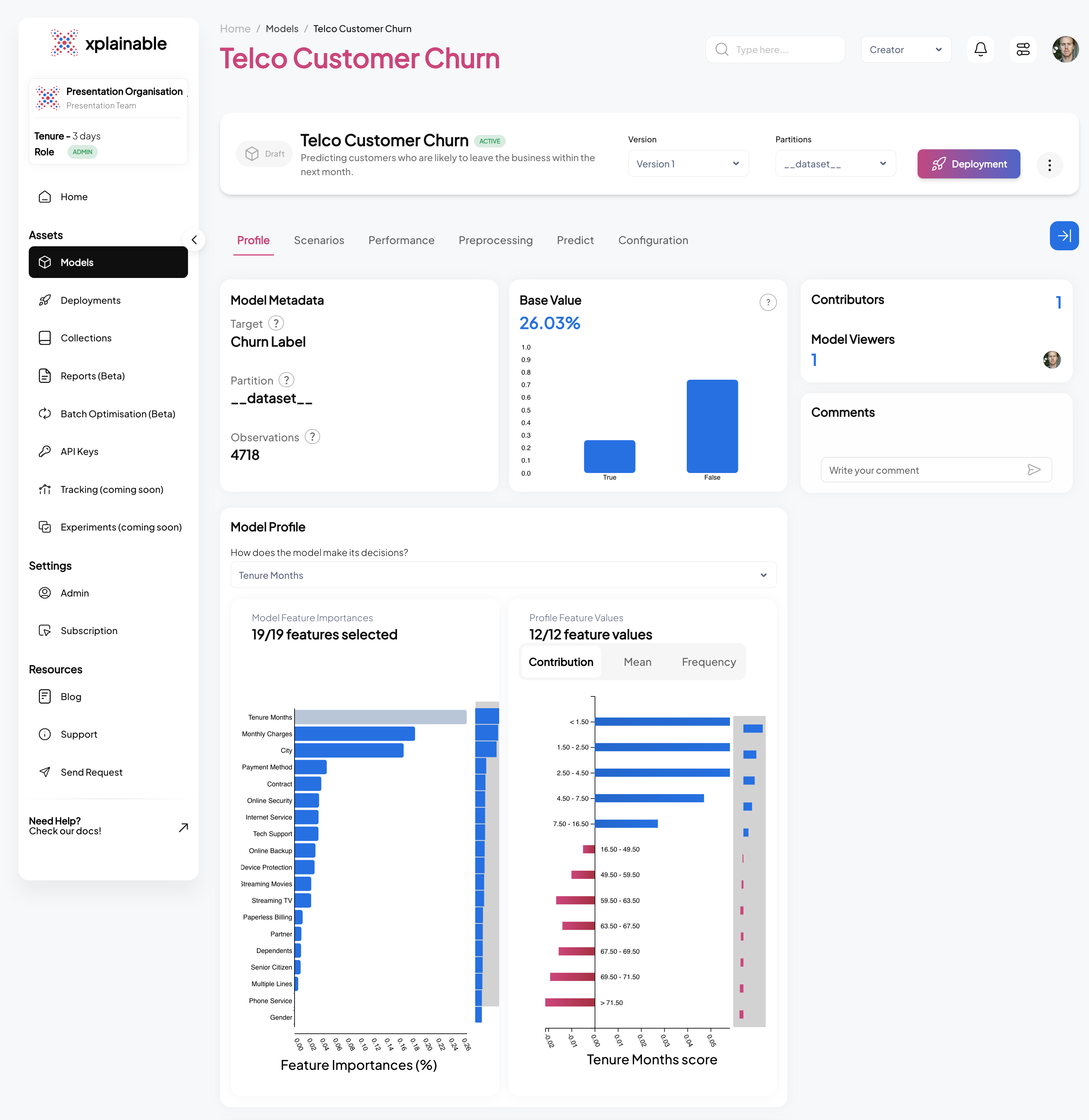
The image displays two graphs related to a churn prediction model.

On the left is the 'Feature Importances' bar chart, which ranks the features by their ability to predict customer churn. 'Tenure Months' has the highest importance, confirming that the length of customer engagement is the most significant indicator of churn likelihood. 'Monthly Charges' and 'Contract' follow, suggesting that financial and contractual commitments are also influential in churn prediction.

The right graph is a 'Contributions' histogram, which quantifies the impact of a specific feature's values on the prediction outcome. The red bars indicate that higher values within the selected feature correspond to a decrease in the likelihood of churn, whereas the green bars show that lower values increase this likelihood.

The placement of 'Gender' at the bottom of the 'Feature Importances' chart conclusively indicates that the model does not consider gender a determinant in predicting churn, thereby ensuring the model's impartiality regarding gender.

5. Model Persisting

In this step, we first create a unique identifier for our churn prediction model using xp.client.create_model_id. This identifier, shown as model_id, represents the newly instantiated model which predicts the likelihood of customers leaving within the next month. Following this, we generate a specific version of the model with xp.client.create_model_version, passing in our training data. The output version_id represents this particular iteration of our model, allowing us to track and manage different versions systematically.

model_id = xp.client.create_model_id(
    model,
    model_name="Telco Customer Churn",
    model_description='Predicting customers who are likely to leave the business within the next month.'
)
model_id

Out:

'CxdKyfllkLMKQYT9'

version_id = xp.client.create_model_version(
    model,
    model_id,
    X_train,
    y_train
)
version_id

Out:

  0%|          | 0/19 [00:00<?, ?it/s]
'3RmCOzUFTtBi5uVX'

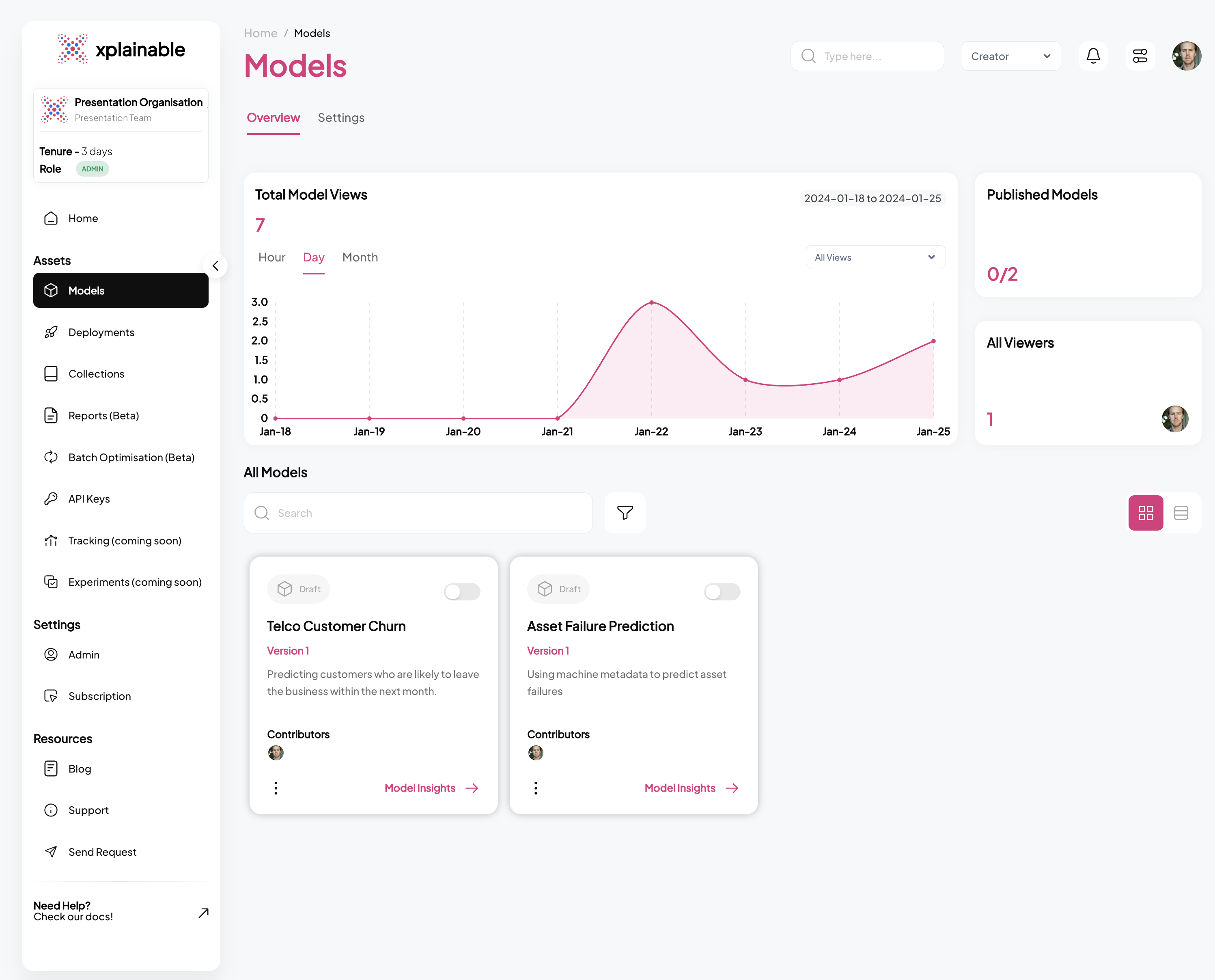
SaaS Models View

Model Image

SaaS Explainer View

Model Image

6. Model Deployment

The code block illustrates the deployment of our churn prediction model using the xp.client.deploy function. The deployment process involves specifying the hostname of the server where the model will be hosted, as well as the unique model_id and version_id that we obtained in the previous steps. This step effectively activates the model's endpoint, allowing it to receive and process prediction requests. The output confirms the deployment with a deployment_id, indicating the model's current status as 'inactive', its location, and the endpoint URL where it can be accessed for xplainable deployments.

deployment = xp.client.deploy(
    hostname="https://inference.xplainable.io", #<- Can set up deployments to be hosted on-prem
    model_id=model_id, #<- Use model id produced above
    version_id=version_id #<- Use version id produced above
)

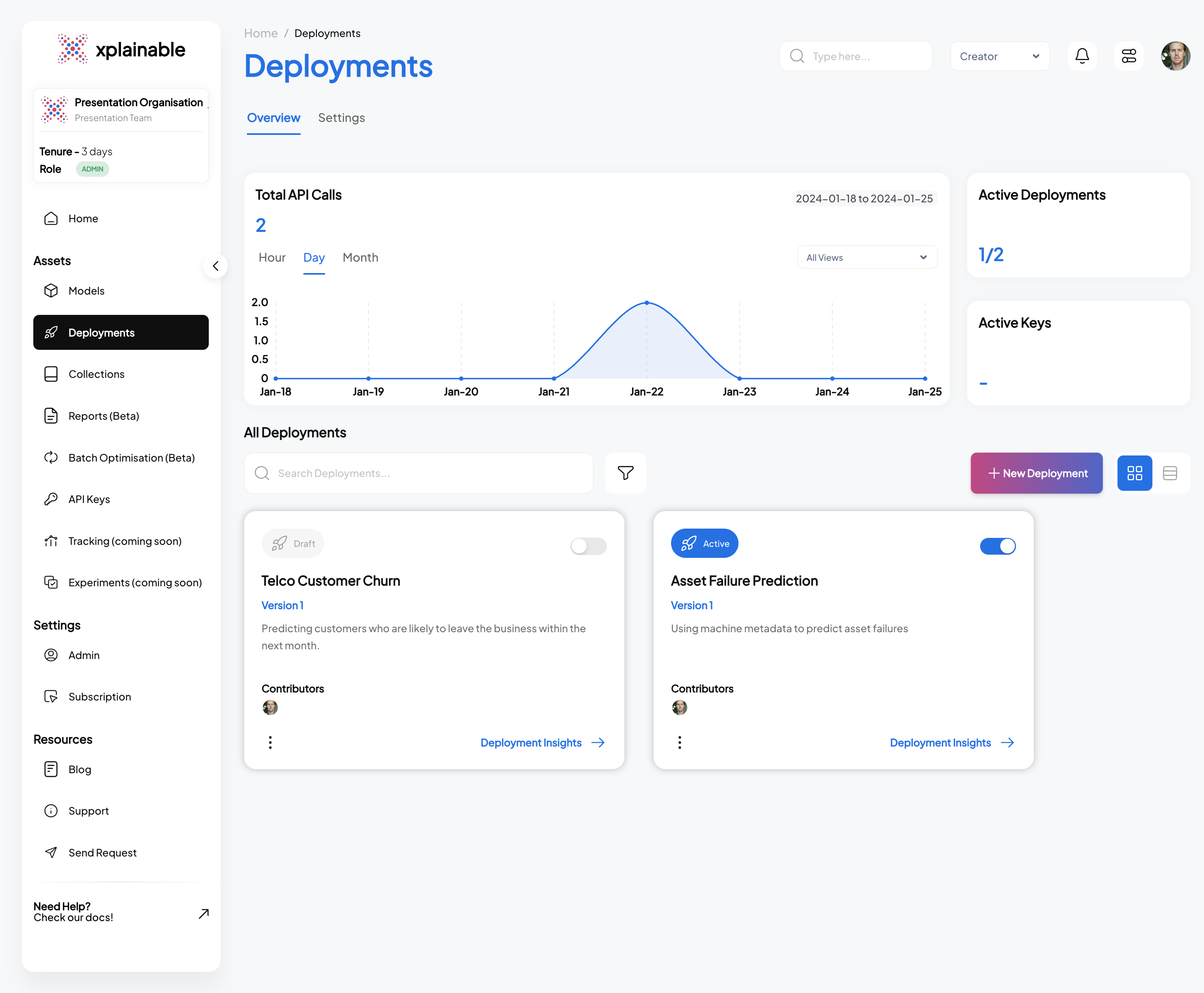
SaaS Deployment View

Model Image

Testing the Deployment programatically

This section demonstrates the steps taken to programmatically test a deployed model. These steps are essential for validating that the model's deployment is functional and ready to process incoming prediction requests.

Activating the Deployment: The model deployment is activated using xp.client.activate_deployment, which changes the deployment status to active, allowing it to accept prediction requests.

xp.client.activate_deployment(deployment['deployment_id'])

Out:

{'message': 'activated deployment'}

Creating a Deployment Key: A deployment key is generated with xp.client.generate_deploy_key. This key is required to authenticate and make secure requests to the deployed model.

deploy_key = xp.client.generate_deploy_key('for testing', deployment['deployment_id'], 7, clipboard=False)

Generating Example Payload: An example payload for a deployment request is generated by xp.client.generate_example_deployment_payload. This payload mimics the input data structure the model expects when making predictions.

#Set the option to highlight multiple ways of creating data
option = 1

if option == 1:
    body = xp.client.generate_example_deployment_payload(deployment['deployment_id'])
else:
    body = json.loads(df_transformed.drop(columns=["Churn Label"]).sample(1).to_json(orient="records"))
    body[0]["Gender"] = None #<- Won't require this line the next release of xplainable

body

Out:

[{'City': 'other',

'Gender': 'male',

'Senior Citizen': 'yes',

'Partner': 'no',

'Dependents': 'yes',

'Tenure Months': 71.5,

'Phone Service': 'no',

'Multiple Lines': 'no',

'Internet Service': 'dsl',

'Online Security': 'no internet service',

'Online Backup': 'yes',

'Device Protection': 'no',

'Tech Support': 'yes',

'Streaming TV': 'yes',

'Streaming Movies': 'no',

'Contract': 'month-to-month',

'Paperless Billing': 'yes',

'Payment Method': 'bank transfer (automatic)',

'Monthly Charges': None}]

Making a Prediction Request: A POST request is made to the model's prediction endpoint with the example payload. The model processes the input data and returns a prediction response, which includes the predicted class (e.g., 'No' for no churn) and the prediction probabilities for each class.

response = requests.post(
    url="https://inference.xplainable.io/v1/predict",
    headers={'api_key': deploy_key['deploy_key']},
    json=body
)

value = response.json()
value

Out:

[{'index': 0,

'id': None,

'partition': '__dataset__',

'score': 0.3928926246322737,

'proba': 0.11276893943031227,

'pred': '0',

'support': 303,

'breakdown': {'base_value': 0.2602797795676134,

'City': -0.0004814338695100573,

'Gender': -7.276610831867163e-05,

'Senior Citizen': 0.045826964522160306,

'Partner': 0.022065879046674532,

'Dependents': -0.01868614293728342,

'Tenure Months': -0.019222955135197697,

'Phone Service': -0.003697016407864983,

'Multiple Lines': -0.0014877658362602538,

'Internet Service': -0.007278086066799008,

'Online Security': -0.017775137133722977,

'Online Backup': -0.0046493037837984,

'Device Protection': 0.0422769557287958,

'Tech Support': -0.009955151311174023,

'Streaming TV': 0.011069611702865327,

'Streaming Movies': 0.024447731368512055,

'Contract': 0.05457342511379243,

'Paperless Billing': 0.024703763630477254,

'Payment Method': -0.009045727458687864,

'Monthly Charges': 0.0}}]

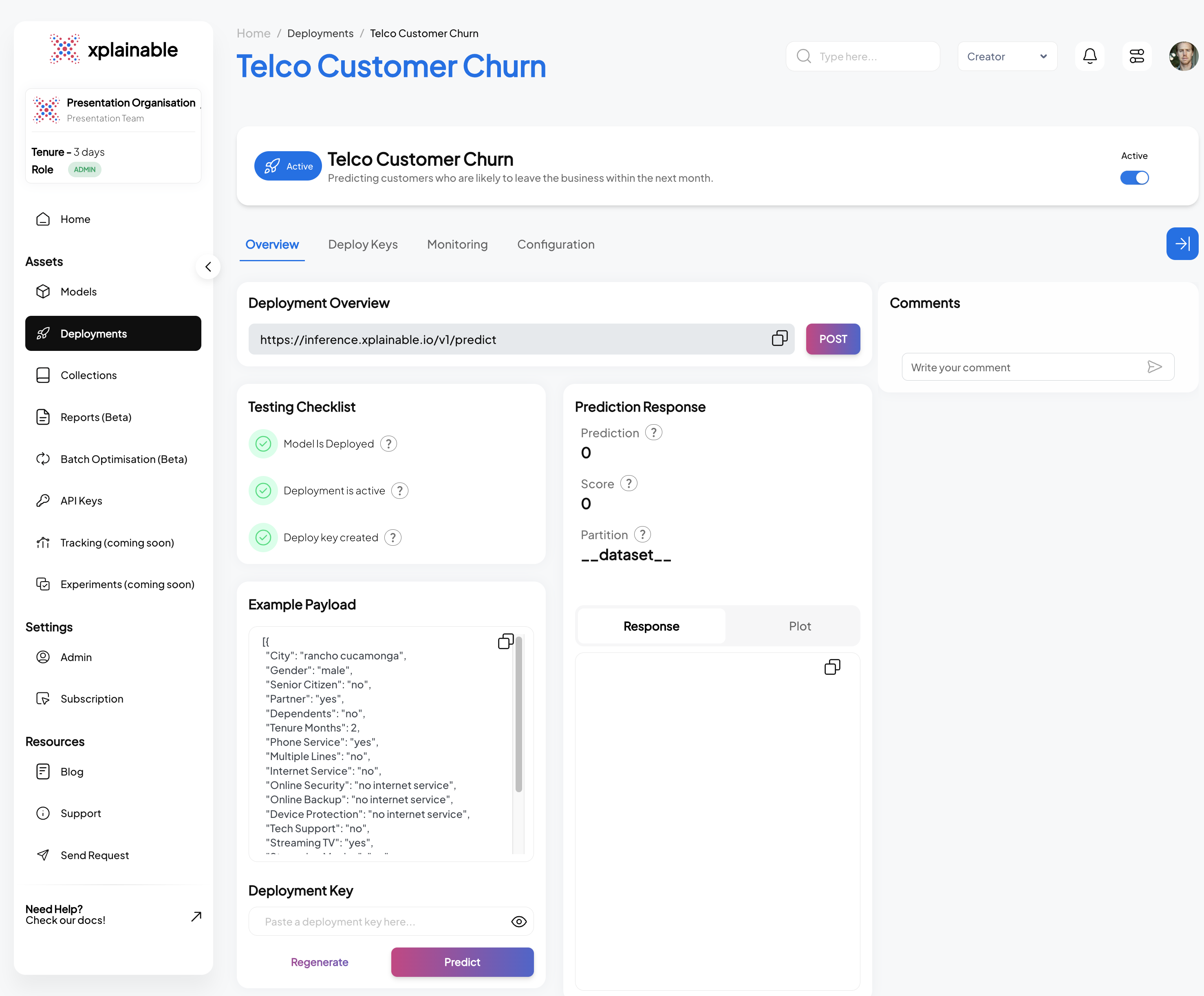
SaaS Deployment Info

The SaaS application interface displayed above mirrors the operations performed programmatically in the earlier steps. It displays a dashboard for managing the 'Telco Customer Churn' model, facilitating a range of actions from deployment to testing, all within a user-friendly web interface. This makes it accessible even to non-technical users who prefer to manage model deployments and monitor performance through a graphical interface rather than code. Features like the deployment checklist, example payload, and prediction response are all integrated into the application, ensuring that users have full control and visibility over the deployment lifecycle and model interactions.

Model Image

7. Batch Optimisation (Beta)

The concept of Batch Optimization within the Xplainable platform represents a significant leap forward from traditional machine learning approaches. Moving away from the prediction -> monitor model approach, this feature offers a dynamic and cost-effective utilisation of model insights.

This optimisation approach allows for the association of monetary costs with various predictive scores. It provides a detailed understanding of the financial impact of different predictive outcomes. For example, within our Telco model, the choice to provide tech support carries a different cost implication than opting against it, influencing the decision-making process.

Features may be fixed or adjustable to align with business requirements. Certain attributes like 'Senior Citizen', 'Tenure', and 'Monthly Charges' may be set due to regulatory standards or business limitations, ensuring that optimisation adheres to these rules.

Conversely, features such as 'Streaming Movies' or 'Device Protection' are modifiable, enabling the exploration of various combinations to discover the most cost-effective approach. The model could assess if altering the contract type for specific customer segments improves retention without markedly raising costs.

Employing the Xplainable model's output in this manner allows organisations to extend past simple predictions to genuine cost optimisation, facilitating strategic decision-making that evaluates each recommended action not only for its impact on outcomes like churn but also for cost-efficiency. Thus, Xplainable's strategy provides businesses the capability to optimise their resources with foresight rarely seen in traditional machine learning.

Package Imports​

Instantiate Xplainable Cloud​

Read IBM Telco Churn Dataset​

Sample of the IBM Telco Churn Dataset​

1. Data Preprocessing​

Turn Label into Binary input​

Preprocessed data​

Create preprocessor ID to persist to Xplainable Cloud​

Link a preprocessor version to the ID​

Loading the Preprocessor steps​

Create Train/Test split for model training validation​

2. Model Optimisation​

3. Model Training​

4. Model Interpretability and Explainability​

5. Model Persisting​

SaaS Models View​

SaaS Explainer View​

6. Model Deployment​

SaaS Deployment View​

Testing the Deployment programatically​

SaaS Deployment Info​

7. Batch Optimisation (Beta)​

Package Imports

Instantiate Xplainable Cloud

Read IBM Telco Churn Dataset

Sample of the IBM Telco Churn Dataset

1. Data Preprocessing

Turn Label into Binary input

Preprocessed data

Create preprocessor ID to persist to Xplainable Cloud

Link a preprocessor version to the ID

Loading the Preprocessor steps

Create Train/Test split for model training validation

2. Model Optimisation

3. Model Training

4. Model Interpretability and Explainability

5. Model Persisting

SaaS Models View

SaaS Explainer View

6. Model Deployment

SaaS Deployment View

Testing the Deployment programatically

SaaS Deployment Info

7. Batch Optimisation (Beta)